Flink-based Web Crawler Talk at Flink Forward 2018

February 19, 2018

On April 10th, at 11am, I’ll be presenting at talk at this year’s Flink Forward conference in San Francisco.

What’s it about? My talk tries to answer the question “Is it possible to build an efficient, focused web crawler using Apache Flink?” It’s actually a bit deeper than that – the challenge I set was whether this could be done using ONLY Flink, without adding in additional infrastructure.

Which took us down some interesting rabbit holes, including fun with iterations, async functions, custom state management, and beating the crap out of the Common Crawl datasets hosted by AWS on S3.

I hope to see some of you there, I promise to make the talk short, entertaining and informative. As opposed to this diagram of the crawler’s workflow…

flink-crawler DAG

ApacheCon Big Data 2016

May 28, 2016

Earlier this month I flew to Vancouver, a wonderful city I’d never had the chance to visit. My excuse was that I was giving a talk at this year’s ApacheCon Big Data conference, which took place in Vancouver from May 9th to 12th.

Ken Krugler ApacheCon

Part of the fun of attending a conference like this is the chance to meet people I’d only interacted with via email. For example, Nick Burch is a super-active Tika committer, so I got to say hi while sitting in on his talk about What’s new in Tika 2.0.

My talk was on creating faster ETL workflows using Cascading and the Cascading-Flink planner to target Flink on YARN. I think that’s enough buzzwords for one post. Net-net was a 50% increase in speed for an ETL workflow that was (in some ways) a worst case for Flink – specifically many grouping/joining operations where the data doesn’t fit in memory, so significant spilling to disk. My slides are up on Slideshare.

Fuzzy matching at Scale

October 18, 2014

In the last few months I’ve given two different talks about scalable fuzzy matching.

The first was a Strata in San Jose, titled Similarity at Scale. In that talk I focused mostly on techniques for doing fuzzy matching (or joins) between large data sets, primarily via Cascading workflows.

More recently I presented at Cassandra Summit 2014, on Fuzzy Entity Matching. This was a different take on the same issue, where the focus was ad hoc queries to match one target against a large corpus. The approach I covered in depth was to use Solr queries to create a reduced set of candidates, after which you could apply typical “match distance” heuristics to re-score/re-rank the results.

The video for this second talk is freely available (thanks, DataStax!) and you can watch me lead off with an “uhm” right here.

Text feature selection for machine learning – part 2

July 21, 2013

In my previous blog post on text feature selection, I’d covered some of the key steps:

  1. Extract the relevant text from the content.
  2. Tokenize this text into discrete words.
  3. Normalize these words (case-folding, stemming)

(and a bit of filtering out “bad words”).

In this blog post I’m going to talk about improving the quality of the terms. But first I wanted to respond to some questions from part 1, about how and why I’m using Cascading and Solr.

Cascading workflow

We use Cascading to create most of our data processing workflows on top of Hadoop, including the sample code for this series of blog posts.

The key benefits are (a) it’s easier to create reliable, high performance workflows and (b) we can use the Cascading local mode to quickly run small data tests locally. In the code I’d posted previously, and below, I typically use unit test routines to process the (relatively) small amounts of test data using Cascading’s locale model

But sometimes you need to process data at scale, using the full power of a Hadoop cluster. I’ve added the TextSimilarityTool, which lets you run the workflow from the command line. To run this tool with Hadoop you’d first build the Hadoop job jar using the ant “job” target:

% ant job

This creates a build/text-similarity-job-1.0-SNAPSHOT.jar file suitable for use with Hadoop. Then you could run this via:

% hadoop jar build/text-similarity-job-1.0-SNAPSHOT.jar
    com.scaleunlimited.textsimilarity.TextSimilarityTool 
    -input src/test/resources/mahout-emails.tsv 
    -workingdir build/TextSimilarityTool/working

The actual workflow (generated by adding “-dotfile build/TextSimilarityTool/flow.dot” to the list of TextSimilarityTool parameters, and then opening with OmniGraffle) looks like this:

TextSimilarityFlow

I’ve color-coded the result, so that read/write operations are green, map operations are yellow, and reduce operations are purple. So visually I can see that this is five separate Hadoop jobs.

Solr

So far we’re using Solr to parse the text into words, which has good performance and reasonable results across many different languages.

We could opt for using natural language processing (NLP) to do the parsing. This involves a much deeper and more complex parse of the input text, but you can wind up with better results.

Some options for NLP-based parsing include NLTK & Topia (Python), OpenNLP, LingPipe, GATE, the Stanford NLP components, etc.

The main advantage of an NLP approach is that you can avoid some of the noise in the resulting data (covered below). For example, you can select only nouns and noun phrases as terms, which also means you might get really juicy terms like “Support Vector Machine”, whereas using a bigram approach would give you “support vector” and “vector machine”.

The disadvantages are (a) performance is much worse, (b) there are fewer supported languages, and (c) most NLP packages have problems with text snippets such as email subjects, page titles and section headers, where you often wind up with sentence fragments.

In a future blog post I’ll talk about using Solr to actually generate similarity scores, which can be a powerful technique, especially for real-time recommendation systems.

Tuning up terms

We’ve got some terms, but there’s clearly more work to do.

There are various approaches to filtering, which we’ll discuss in more detail in part 3 (e.g. filter by a minimum LLR score)

But before we start pruning data, we want to expand our features by adding terms with two words (phrases), as that often adds more useful context. Some people talk about this as bigrams, or as “shingles” with a size of 2.

The SolrAnalyzer is already set up to generate multi-word phrases, via the alternative constructor that takes a shingle size. If we set the size to 2, then we’ll get all one and two word combinations as terms. For example, “the quick red fox” becomes “the”, “quick”, “the quick”, “red”, “quick red”, “fox”, “red fox”.

With this change, our results look a bit different. To generate this output, I’m using the testBigrams() method in TextSimilarityWorkflowTest, and (from Eclipse) setting the JVM size to 512MB via -Xmx512m. Note that I’m now processing the mahout-emails-big.tsv file, to get sufficient context for more sophisticated analysis. Running testBigrams() and then opening up the resulting build/test/TextSimilarityWorkflowTest/testBigrams/working/terms/part-00000 file and getting terms for the ted.dunning@gmail.com email user gives me:

u_k	14.23436727499713
gmail.com wrote	13.511520087344097
that	13.18694502194829
v_k	11.742344990218701
sgd	10.54641662066267
regress	10.422268718215433
wrote	10.382580653619346
gmail.com	10.362437176043924
veri	9.924853908087771
iri	9.534937403528989
categori	9.481973682609356
u_k u_k	9.448681054284984

Now we have a new problem, though. We get phrases that are unexpected (high LLR score) but intuitively don’t add much value, such as “gmail.com wrote”. Typically these are phrases with one or two common words in them. We could use a stop word list, but that’s got a few issues. One is that you’ll find yourself doing endless manual tweaking of the list, in the hopes of improving results.

The other is that the stop word list from Lucene (as one example) is a very general list of terms, based on analysis of a large corpus of standard text. For our example use case, the word “mahout” might well turn out to be noise that should be excluded.

So how should we go about figuring out the list of terms to exclude? One common technique we use is to generate document frequency (DF) values for terms, and then visualize the results to pick a cutoff. All terms with DF scores higher than this cutoff go into the “bad terms” (aka stop words) list. Once we have this list, the SolrAnalyzer is already set up to exclude matching terms, and also to not emit any phrases that contain a stop word.

Since this stop words list is needed by the SolrAnalyzer, it has to be created by an upstream workflow. The StopwordsWorkflow code handles this for us. It will generate a list of stop words if you provide a -maxdf (maximum DF score) parameter, or in the absence of this parameter it will output the top 2000 terms, sorted by their DF score, for use in visualizing results. Note that here we want to parse and extract only single-word terms.

If we run this workflow without the -maxdf parameter, we’ll get a file that contains tab-separated word and DF results useful for visualization. For example, the testTopDFTerms() method in StopwordsWorkflowTest creates the file build/test/StopwordsWorkflowTest/testTopDFTerms/working/terms-by-df/part-00000 which has the terms:

the     0.96816975
mahout  0.9018568
and     0.9005305
for     0.8633952
thi     0.82626
thank   0.8222812
with    0.7997348
that    0.79708225
have    0.7798408
can     0.74005306

As you can see, “mahout” is indeed a very common term, appearing in emails written by 90% of all users (remember that we’re treating as a “document” the aggregate of all emails written by a given user, based on the email address). And “thank” is in emails written by 82% of all users, so the list seems reasonably polite 🙂

It’s curious that “the” isn’t in emails written by 4% of the users. I’d guess that this happens when a user writes emails that we can’t parse, and thus we get an empty email body. One easy way to dig into this is to generate a Solr index with the text being analyzed, which I might do for the next blog post.

In any case, dropping this into Excel we get…

word df graph

The Y-axis is the DF (document frequency), which varies from 0 to 1.0. The X-axis is just the term rank, from 1 (the term with the highest DF score, which is “the” in our example) down to 2000. This exhibits the happy power curve shape we’d expect. I typically pick a max DF score that’s right at the “elbow”, which is about 0.20 in the above graph. Interestingly enough, this 0.2 value is often the cut-off value for DF that I wind up using, regardless of the actual dataset being processed.

Now we can re-run the workflow, this time with the -maxdf 0.20 parameter and get a stop words list that we pass to the SolrAnalyzer constructor. We could automate the above process, by doing some curve fitting on the results and detecting the elbow, but for typical workflows the nature of the incoming data doesn’t change that much over time, so leaving it as a manual process is OK. I’ve added the list of stop words as src/main/resources/stopwords.txt. The last five terms in this file are:

fri
singl
those
expect
final

And those all seem reasonable to treat as stop words. Note that these are normalized (e.g. stemmed) terms, so you wouldn’t be able to directly use them as typical Solr/Lucene stop words. Instead the SolrAnalyzer code applies these against the analyzed results. In addition, this list wants to be language-specific. In fact much of the text processing (tokenizing, stemming, etc) should vary based on the language. Maybe that’s a topic for a future blog post series…

With our stop words list, we can regenerate results using the testStopwords() method in TextSimilarityWorkflowTest, which now look significantly better.

u_k	14.332966007716099
v_k	11.823697055234904
sgd	10.717215693020618
regress	10.58641818402347
categori	9.706156080342279
iri	9.675301677735192
u_k u_k	9.512846458340425
histori	8.913169188568189
dec	8.876447146205434
averag distanc	8.748071855787957

Filtering

At this point in the process we’re faced with a decision about second-stage filtering. Previously we’d filtered out noise (short words, numbers, stop words). Now we could do additional filtering to reduce the number of terms per document.

The first question is why might we want to do any filtering. The most common reason is one of performance – in general, fewer features mean better performance with machine learning algorithms, regardless of whether we’re doing k-means clustering or Solr-based real time similarity. Depending on what’s happening downstream, it might also make sense to reduce the amount of data we’re running through our workflow, which again is a performance win.

The second question is how to filter. There are lots of options, including:

  • Picking a minimum LLR score (which might vary by the number of words in a term)
  • Using a feature-reduction algorithm such as SVD (Singular Value Decomposition).
  • Calculating a TF*IDF (Term frequency * inverse document frequency) score and taking only the top N.

It can also make sense to combine different types of filters – for example, to filter by a minimum LLR score initially to reduce the number of terms (workflow optimization), then calculate another score such as TF*IDF on the remaining terms.

In the next blog post, we’ll use TF*IDF to pick the best terms for each user, but we’ll do it in a way that is optimized for similarity. Stay tuned, I’ll try to get that written before I disappear for two weeks on the John Muir Trail.

Text feature selection for machine learning – part 1

July 10, 2013

We do a lot of projects that require extracting text features from documents, for use with recommendation systems, clustering and classification.

Often the “document” is an entity like a person, a company, or a web site. In these cases, the text for each document is the aggregation of all text associated with each entity – for example, it could be the text from all pages crawled for a given blog author, or all tweets by one Twitter user.

This seemingly trivial aspect of a big, sophisticated machine learning-based project is often the most important piece that you need to get right. The old adage of “garbage in, garbage out” is true in spades when generating features for machine learning. It doesn’t matter how cool your algorithm is, your results will stink if the features don’t provide good signals.

So I decided to write up some of the steps we go through when generating text-based features. I’m hoping you find it useful – please provide feedback if anything isn’t clear, or (gasp) isn’t correct.

Similarity

In order to constrain this writing project to something a bit less overwhelming, I’m going to focus on just one aspect of machine learning & text features, namely similarity. Often similarity between two entities is the “distance” between their feature vectors, which is a set of attributes and weights. The closer these two feature vectors are to each other, the greater the similarity between the two entities.

For example, if I’ve got two users, and the first user’s name is “Bob Krugler” and the second user’s name is “Krugler, Robert”, I could calculate a similarity between them based on equality (or lack thereof) between the names. The feature vector for each user consists of names and weights, such as [Bob:1, Krugler:1] and [Robert:1, Krugler:1]. I could get better results by doing things like synonym expansion, such that “Bob” is equal to “Robert”. Note that using this approach, I’d say that “Joe Bob” was somewhat similar to “Bob Krugler”, since they’ve got the name “Bob” in common, even though for “Joe Bob” this is (supposedly) a last name. Which actually might be a good thing, if you’re dealing with badly formatted input data.

Using text as features for calculating similarity between entities makes sense, and is a common approach for content-based recommendation engines. The other main approach for recommendations is collaborative filtering, where the user’s relationship with items (e.g. user activity) determines whether two users or items are similar (e.g. “how many books did user X and user Y both view?”).

Content-based similarity is especially useful when you don’t have much user activity data to derive similarity, or the lifespan of an item (or a user) is so short that there isn’t a lot of overlap in user-item activity, and thus it’s hard to find similar users based on shared preferences for items.

The power of content-based similarity is that once I have an effective way to create good features and meaningful weights, I’m in a good position to do clustering of users, recommend emails to read, recommend users to connect with, etc. And I can do all of this without any user-item preferences.

But picking the right set of text features to use for content-based similarity isn’t easy, and in this series of blog posts I’ll try to walk you through the typical sequence of steps, using as our example data set the emails posted by users to the Mahout mailing list. If we have good features, we should be able to calculate appropriate similarity scores (distances) between users.

The code and data used in my write-up can be found at http://github.com/ScaleUnlimited/text-similarity. As the code will be evolving while I write these blog posts, I’ll be creating tags named “part 1”, “part 2”, and so on.

One final note – I’m using Cascading to define the workflows that generate my features, Solr/Lucene to extract words from text, and Mahout to find similar users. But the actual systems used to generate features and calculate similarities matter less than the process of figuring out how to get good features out of the text.

Getting the data

The first step is always collecting the data we’re going to use in the analysis. I grabbed the archive page at http://mail-archives.apache.org/mod_mbox/mahout-user/, extracted all of the links to archive files (in the mbox format), and then downloaded all of the files.

After that I needed to generate data in a useful, easy-to-process format for downstream analysis. My target was one line per email, with tab-separated fields for msgId, author, email, subject, date, replyId and content. The Tika content analysis project has an RFC822 parser for parsing these mbox files, but it generates a single output for each file, without some of the fields that we need.

So I first had to write code to split mbox files on email boundaries, and then use a modified version of the Tika RFC822 parser to extract all of the required metadata. I also had to convert tabs and newlines in the text to \t and \n sequences, so as to avoid issues with Hadoop splitting up text files on line boundaries.

The code for this processing is in the com.scaleunlimited.emailparsing package.

The end result is a a file with lines that look like this (fields broken into separate lines):

msgId: <1326798618.75219.YahooMailNeo@web121201.mail.ne1.yahoo.com>
author: Harry Potter
email: harry456great@yahoo.com
subject: Re: MR Vectorization
date: 2012-01-17T11:10:18Z
replyId: <4F155317.1070703@gmail.com>
content: thanks sir...  that was really helpful..\n\n\n...

There are two versions of this data in the GitHub project, one with only 100 emails called mahout-emails.tsv, and the other with 5900 emails called mahout-emails-big.tsv.

Generating text features

Now we come to the heart of the matter – what makes a good text feature for calculating similarity? There’s no single approach that works in all situations, but some common steps that you almost always need are:

  1. Extract the relevant text from the content.
  2. Tokenize this text into discrete words.
  3. Normalize these words (case-folding, stemming)
  4. Filter out “bad words”.
  5. Generate terms from multiple adjacent words.
  6. “Boost” terms based on structure.
  7. Aggregate terms for entities and generate term scores.
  8. Filter terms to reduce feature “noise”.

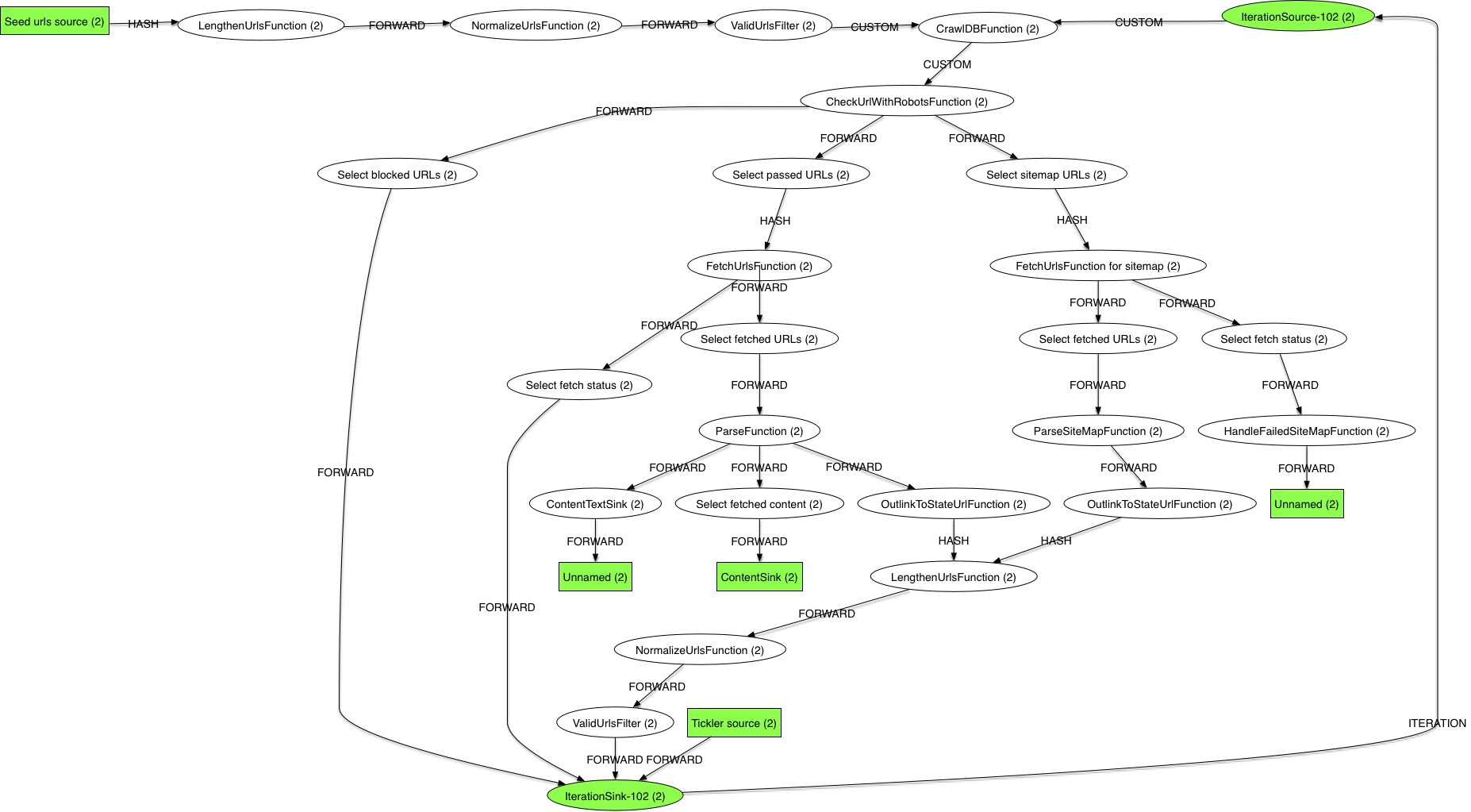
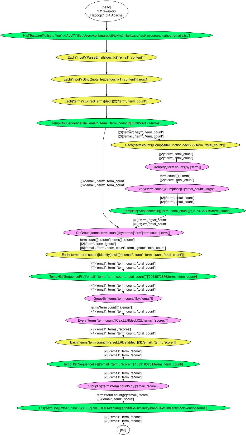
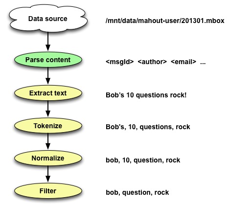
I’ll cover steps 1, 2, 3 & a bit of 4 in the remainder of this blog post, the rest of step 4 in part 2, and steps 5 through 8 in part 3. The portion of the overall workflow that we’re discussing here looks like…

Pipeline

Step 1 – Extracting relevant text

We’ve got two fields with interesting text – the subject, and the content.

For this step, we’re going to focus on just the content – we’ll talk about the subject field in step 6, in the context of boosting terms based on structure.

This step is trivial, primarily because the heavy lifting of parsing mail archives has already been done. So we have a field in our input text which has exactly the text we need. However we need to re-convert the text to contain real tabs and linefeeds, versus the escaped sequences, as otherwise that messes up the tokenization we’ll be doing in the next step (e.g. the sequence “\tTaste” would be tokenized as “tTaste”, not just “Taste”). There’s a ParseEmails function in the TextSimilarityWorkflow.java file which takes care of this step.

Initially I thought that I should also strip out quoted text from email, since that wasn’t text written by the email author, but it turns out that’s often very useful context. Many reply-to emails are mostly quoted text, with only small amounts of additional commentary. The fact that the email author is replying to an earlier email makes all of the text useful, though we might want to apply weighting (more on that in step 6).

Step 2 & 3 – Tokenizing & normalizing text

Now we’re into the somewhat arcane area of text analysis. Generally this is a series of transformations applied to a large “chunk” of text, which includes:

  • Splitting the text into discrete tokens (tokenization).
  • Simple normalization such as lower-casing and removing diacriticals.
  • Stemming and other language-specific transformations.

Luckily Solr (via Lucene) has support for all of these actions. We could directly use Lucene, but building our analysis chain using Solr makes it easy to configure things using XML in the schema.xml file. For example, here’s a field type definition for English text:

    <fieldType name="text_en" class="solr.TextField">
      <analyzer>
        <tokenizer class="solr.StandardTokenizerFactory"/>
        <filter class="solr.ICUFoldingFilterFactory"/>
	    <filter class="solr.EnglishPossessiveFilterFactory"/>
        <filter class="solr.KeywordMarkerFilterFactory" protected="protwords_en.txt"/>
        <filter class="solr.PorterStemFilterFactory"/>
      </analyzer>
    </fieldType>

This says we’re going to do the initial splitting of text into tokens using the StandardTokenizer, then we’ll use the ICUFoldingFilter to make everything lower-case, remove diacriticals, etc. After that we’ll strip out possessives, then we’ll set up for Porter stemming by protecting words that shouldn’t be stemmed.

But how do we use Solr in a Cascading/Hadoop workflow? The SolrAnalyzer class has the grungy details, but basically we synthesize what looks like a Solr conf directory, using resources found inside of our jar (in src/main/resources/solrparser), and then we can instantiate a Lucene Analyzer based on our target field type (e.g. “text_en”).

So how well does this work? If we pass in “Bob’s questions rock!” to the analyzer, we’ll get back “bob”, “question”, “rock” – so that’s pretty good.

Things can get a bit wonky with stemming, though. If we analyze “feature category” we’ll get back “featur” and “categori”, which can be a surprise. For cases where the stemming is too aggressive (and it stems two unrelated words to the same base form), you can add entries to the “protwords_en.txt” file to protect them from modification by the stemming algorithm.

Step 4 – Filtering

Often you’ll wind up with terms (words) that are clearly not going to be very useful as text features. But how do you go about identifying significant bad terms and then removing them?

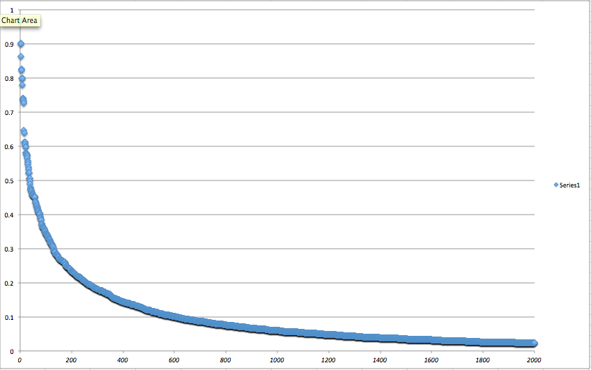
The first thing we often do is calculate a log-likelihood ratio (LLR) score for every term, and sort the results. This lets us eyeball things quickly,  tweak settings, and repeat the process. So what’s a log-likelihood ratio? It’s basically a measure of how unlikely it is that some event would have occurred randomly. In our case, it’s how unlikely a given word could have occurred as many times as it did, in emails written by one user, when compared to all words written by all user in all emails. For some additional color commentary check out Ted Dunning’s Surprise and Coincidence blog post.

So the higher the LLR score for a word, the more unlikely it is to have randomly occurred as many times as it did, and this then gives us a useful way to sort words. We use a Cascading SubAssembly from our cascading.utils project called TopTermsByLLR to do most of the work for us.

We can run our workflow on the small set of Mahout emails by executing the TextSimilarityWorkflow.test() method, and then opening up the resulting file in “build/test/TextSimilarityWorkflowTest/test/working/terms/part-00000”. If we check out the top words for the ted.dunning@gmail.com email user, we get an unpleasant surprise – almost all of the top terms are noise:

v3	6.981227896184893
3	6.782776936019315
v2	6.497556317809991
q	6.078475518110127
0.00000	6.055874479673747
wiki	5.959521694776826
result	5.9469144102884295
qr	5.93635582683935
liu	5.353852995656953
v1	5.19438925914239

I say this is a surprise, but in reality almost every time you get initial results back, you’re going to be disappointed. You just have to roll up your sleeves and start improving the signal-to-noise ratio, which usually starts with getting rid of noise.

Looking at these results, we could clean things up pretty quickly by ignoring words that were less than 3 characters long, and skip anything that’s just a number (including ‘.’ and ‘,’ characters). There are a number of places we could do this filtering, but eventually we’ll need to handle it inside of the SolrAnalyzer class when we start generating multi-word terms. The filterWord method is the right modification point, and once we’ve changed it to exclude short words and numbers, our results improve a bit:

result	6.299652144395367
wiki	6.220453017016188
liu	5.553637211267486
mymail	5.050533090688624
as.matrix	4.51710231608846
liuliu.tju	4.501488208584039
decomposit	4.431912003379223
score	4.266076943795874
gmail.com	4.263470592109653
exactli	4.178110810351496

We still get words like “result” that seem pretty generic, and words like “liuliu.tju” that look junky, but we’re probably close enough to start thinking about more sophisticated filtering and actual term scoring.

Stay tuned for part two…

The Durkheim Project goes live!

July 3, 2013

As of today, the Durkheim Project is now live. This is a research project involving Patterns and Predictions, the Geisel School of Medicine at Dartmouth, the U.S. Department of Veterans Affairs (VA) and Facebook. See the Durkheim Project launch announcement for full details.

Durkheim Project

The worthy goal of the Durkheim Project is to improve the medical community’s ability to predict suicides. The driving force was original the military’s concern about increasing suicide rates among service personnel, which is why DARPA funded the initial phase of the project. However the CDC recently released a report based on 10 years of suicide data in the US that clearly shows this is a problem for all Americans.

We were a (small) part of the project, implementing both the Cassandra-based data capture system being used by the Facebook app, and Cascading-based workflows to apply predictive analytics models at scale to social media data. I gave a talk at the 2013 Cassandra Summit on the project.

To participate in the Durkheim Project, please go to https://apps.facebook.com/durkheimsocial/

Large scale analytics using Hadoop and Solr

April 3, 2013

I finally got around to posting the slides from last year’s talk I gave at Hadoop Summit.

The focus of the presentation was about how we used Hadoop & Solr to solve a big data analytics problem for one of our clients.

They have a web site that helps advertisers target publishers/networks and improve ad results by analyzing millions of web pages every day. They were able to cut monthly costs by more than 50%, improve response time by 4x, and quickly add new features by switching from a traditional DB-centric approach to one based on Hadoop & Solr. This analysis is handled by a complex Hadoop-based workflow, where the end result is a set of unique, highly optimized Solr indexes. The data processing platform provided by Hadoop also enables scalable machine learning using Mahout.

This presentation some of the unique challenges in switching the web site from relying on slow, expensive real-time analytics using database queries to fast, affordable batch analytics and search using Hadoop and Solr.

Faster Tests with Cascading 2.0 Local Mode

October 22, 2012

For one of our clients, we’d developed a series of complex workflows using Cascading 1.2 that get run multiple times every week, using Amazon’s Elastic MapReduce. These 15 or so higher-level workflows get planned by Cascading into 80+ Hadoop jobs, which Cascading takes care of running for us. That part has been working well, and the end result (a set of Solr indexes) powers the Adbeat web site.

But we’ve had to struggle with how long our tests take. Because of the way we combine & aggregate results, and the inter-connected nature of various workflows, we have to pump a fair amount of data through the complete process in order to validate that we get the expected end results.

And that in turn meant our pre-deploy tests were taking close to 90 minutes to complete. So we started cutting corners, by sometimes skipping tests, or beginning a deploy while running tests at the same time…and we all know that’s the path to darkness.

With Cascading 2.0 comes a new workflow planner, something (confusingly) called “local mode”. This isn’t the same as Hadoop local mode, where the Cascading Hadoop planner has generated some number of Hadoop jobs that run locally (how we were running our tests). Instead there’s a new planner that generates a locally executed “plan” for the workflow, without using anything from Hadoop. Based on some quick tests, it was clear that running tests in Cascading local mode would be much faster, by potentially an order of magnitude.

But in order to do that, we’d have to first port our code from Cascading 1.2 to 2.0, and then work around various issues & limitations with Cascading local mode. What follows is a detailed description of the changes we had to make, for anyone else contemplating the same process.

Porting to Cascading 2.0

This was actually pretty easy, for our actual workflows. The one issue we ran into was a change in what our custom Buffers saw in the grouping TupleEntry. Previously with Cascading 1.2 if we were grouping two pipes using an OuterJoin, BufferCall.getGroup() would return just the non-null grouping key field value(s), which we would then access by index. Cascading 2.0’s BufferCall.getGroup always returns the field value(s) from both pipes, which can be accessed by field name. For example, suppose the grouping key is a single field (e.g., with a field named ‘left-key-field’ on the left and ‘right-key-field’ on the right), and the first key has null on the left (i.e., no matching Tuple) and ‘right-key-value’ on the right. Cascading 1.2’s BufferCall.getGroup returns fields: [0] tuple: ['right-key-value'], while Cascading 2.0’s BufferCall.getGroup returns fields: ['left-key-field', 'right-key-field'] tuple: [null, 'right-key-value']. This is better, but it did cause some code to fail, because it was calling getString(0) on the group TupleEntry, and assuming it would always get the non-null grouping key value.

The bigger challenge was in porting to 2.0 all of the other re-usable components we’d created and now relied on. For example, we have a Solr scheme that we use to build the indexes. And there’s a bunch of utility code in the open source cascading.utils project, much of which was dependent on Cascading internals. So all of that had to be ported & tested first.

After about a week of work, we were able to run with Cascading 2.0, though still in Hadoop local mode. That was the good news. The bad news was that tests now took even longer, by about 10 minutes. This was apparently due to the simultaneous change to use Hadoop 1.0.3 vs. Hadoop 0.20.2, where the newer version of Hadoop seems to take longer to set up & tear down each job (at least in local mode). We were able to get back most of this time by using the FlowProps.setJobPollingInterval(200).

Porting to Cascading Local Mode

Now the real fun started. We needed to create a generic platform that let us target either Hadoop (when running in a real cluster) or Cascading Local (during testing/debugging). We wound up adding some support in cascading.utils for this, along with a generic “Path” that we could use for things like enumerating all files or directories in a directory. The BasePlatform class defines a small set of abstract methods, which was the minimum set we needed – your mileage may vary.

    public abstract boolean isLocal();
    public abstract boolean isTextSchemeCompressable();
    public abstract void setNumReduceTasks(int numReduceTasks) throws Exception;
    public abstract void setFlowPriority(FlowPriority priority) throws Exception;
    public abstract FlowConnector makeFlowConnector() throws Exception;
    public abstract FlowProcess makeFlowProcess() throws Exception;
    public abstract BasePath makePath(String path) throws Exception;
    public abstract BasePath makePath(BasePath parent, String subdir) throws Exception;
    public abstract Tap makeTap(Scheme scheme, BasePath path, SinkMode mode) throws Exception;
    public abstract Scheme makeBinaryScheme(Fields fields) throws Exception;
    public abstract Scheme makeTextScheme(boolean isEnableCompression) throws Exception;
    public abstract Scheme makeTextScheme() throws Exception;

You’ll note the calls to makeTextScheme() and makeBinaryScheme(), which help us abstract out the calls to create TextLine and SequenceFile schemes. Since there is no SequenceFile scheme in Cascading local mode, we defined a KryoScheme that is returned by the Cascading local version of makeBinaryScheme().

One of the challenges was that Cascading’s local version of TextLine doesn’t support reading or writing compressed text files, whereas the Hadoop version does (because it’s leveraging Hadoop support for this). So we had to create uncompressed versions of our test data, and avoid assuming that the output of some flows was compressed. We’ve got a pending patch for Cascading that adds back in compression support, which would simplify some of the above support.

We also had to create a Cascading local version of SolrScheme, since Schemes and Taps often are tied to the target platform. And we made a DirectoryTap for local mode, which acts like the Lfs Tap in Hadoop mode – e.g. it supports reading from a directory of files, unlike the FileTap.

Then the tedious work started; we had to modify all of our code to remove any an all references to Hadoop-specific support, and switch over to using this BasePlatform class in all cases. One of the challenges here was that we often cast the generated FlowProcess class into HadoopFlowProcess, to get at Hadoop-specific functionality…and obviously all of those casts would fail at run-time when running in Cascading local mode.

We also wound up having to wrap BasePlatform with another class that contained some generic platform support that was very specific to our use case, e.g. setting specific Elastic MapReduce values when running in Hadoop mode.

And then we got to debug it all. There were only two really tricky issues we ran into…

ThreadLocal – In Cascading local mode, a Function’s prepare() method can be called by one thread, and its operate() method by a different thread. This caused problems with some text parsing code we had, which set up a Lucene reusable token stream in the prepare() method and then used it in the operate() method. The issue is that Lucene uses ThreadLocal to keep track of these reusable token streams, so our carefully prepared stream wasn’t being used by our operate() method.

Tuple cloning – In many of our custom Function and Buffer classes, we reuse a Tuple when emitting results as a way of avoiding lots of memory allocations/GC hell. This works fine in Hadoop, because calling the outputCollector.add() method effectively does a deep clone of the Tuple via serialization before returning. But in Cascading local mode, only a shallow copy is done, and the Tuple is kept around in memory if it’s being used in a subsequent grouping operation. We were stuffing Tuples inside of the Tuple, and thus these mutable objects were not getting cloned. Our quick & dirty solution was to add a static clone() method to our internal Cascading platform class, which we had to use everywhere that we called outputCollector.add(). This would walk the Tuple, and create a deep copy of any mutable objects (though only in Cascading local mode). The problem with our solution is that any new code will also need to remember to use this pattern of outputCollector.add(Platform.clone(theTuple)), otherwise the problem could pop up again.

And the Final Result

In the end, it was worth it – though much harder than we initially expected.

We were able to reduce our test times from 90 minutes to 10 minutes. And at this point it was obvious where we were processing more data than needed, so with a few small changes we further reduced our time down to 4 minutes. So ultimately we got more than a 20x improvement in test time, and we’re back to religiously running tests before committing and code or doing any deployments of jobs.

We still of course have to test against the real Hadoop platform, but that happens as part of our release cycle, where we generate test indexes using samples of real data that are then validated by QA.

Cascading & GigaSpaces

September 11, 2012

We’ve just started a new project, which is to create a “planner” that lets you define & run complex workflows in GigaSpace’s XAP environment, using the Cascading API.

There are lots of interesting challenges, mostly around various impedance mismatches between the Cascading/Hadoop model of data storage and parallel map-reduce execution, versus the in-memory data grid and transactional support provided by GigaSpaces.

Step one has been to create a Cascading Tap that lets a Hadoop-based workflow read from/write to a GigaSpaces “space”, which means one or more partitions in their data grid.

Step two is in progress, and that’s to support running real map-reduce workflows using GigaSpaces XAP.

If we’re successful, we’ll wind up with the ability to run the same workflow in Hadoop (extreme scalability, batch) and GigaSpaces (low latency, incremental) without any changes to the workflow definition.

Presentation at Hadoop Summit 2012

June 11, 2012

I’ll be speaking at the Hadoop Summit conference on Thursday (2:25pm), about how to replace Oracle (or MySQL, etc) with Hadoop + Solr. The title is “Faster, cheaper, better – switching a web site from DB queries to Hadoop & Solr“. It’s a distillation of experience with clients, where we use Hadoop to do off-line pre-processing of data, which then lets us use Solr as a NoSQL solution that provides faster query processing on less hardware, while adding additional search & faceting functionality.