Text feature selection for machine learning – part 2

In my previous blog post on text feature selection, I’d covered some of the key steps:

1. Extract the relevant text from the content.
2. Tokenize this text into discrete words.
3. Normalize these words (case-folding, stemming)

(and a bit of filtering out “bad words”).

In this blog post I’m going to talk about improving the quality of the terms. But first I wanted to respond to some questions from part 1, about how and why I’m using Cascading and Solr.

Cascading workflow

We use Cascading to create most of our data processing workflows on top of Hadoop, including the sample code for this series of blog posts.

The key benefits are (a) it’s easier to create reliable, high performance workflows and (b) we can use the Cascading local mode to quickly run small data tests locally. In the code I’d posted previously, and below, I typically use unit test routines to process the (relatively) small amounts of test data using Cascading’s locale model

But sometimes you need to process data at scale, using the full power of a Hadoop cluster. I’ve added the TextSimilarityTool, which lets you run the workflow from the command line. To run this tool with Hadoop you’d first build the Hadoop job jar using the ant “job” target:

% ant job

This creates a build/text-similarity-job-1.0-SNAPSHOT.jar file suitable for use with Hadoop. Then you could run this via:

% hadoop jar build/text-similarity-job-1.0-SNAPSHOT.jar
    com.scaleunlimited.textsimilarity.TextSimilarityTool 
    -input src/test/resources/mahout-emails.tsv 
    -workingdir build/TextSimilarityTool/working

The actual workflow (generated by adding “-dotfile build/TextSimilarityTool/flow.dot” to the list of TextSimilarityTool parameters, and then opening with OmniGraffle) looks like this:

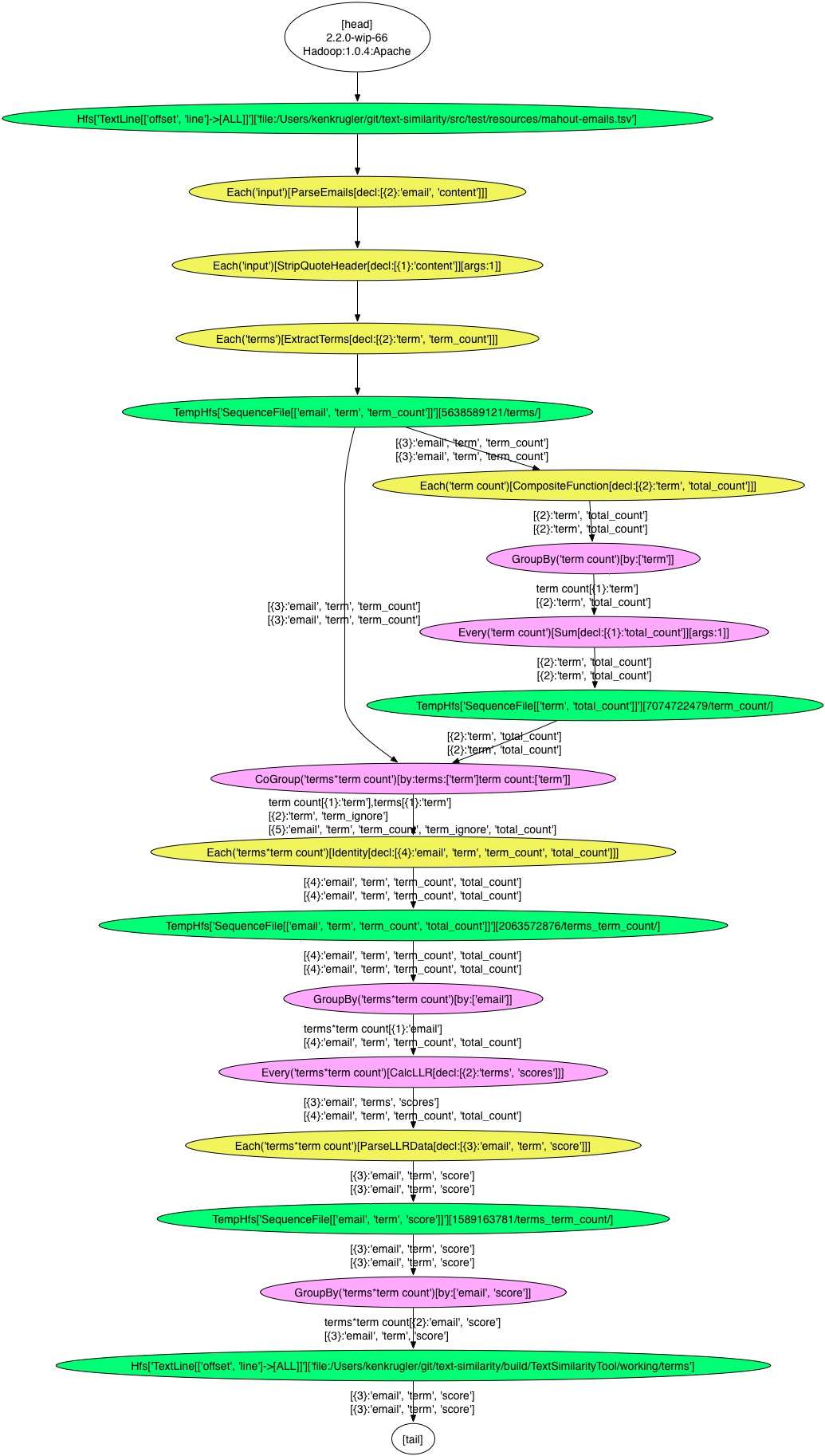
I’ve color-coded the result, so that read/write operations are green, map operations are yellow, and reduce operations are purple. So visually I can see that this is five separate Hadoop jobs.

Solr

So far we’re using Solr to parse the text into words, which has good performance and reasonable results across many different languages.

We could opt for using natural language processing (NLP) to do the parsing. This involves a much deeper and more complex parse of the input text, but you can wind up with better results.

Some options for NLP-based parsing include NLTK & Topia (Python), OpenNLP, LingPipe, GATE, the Stanford NLP components, etc.

The main advantage of an NLP approach is that you can avoid some of the noise in the resulting data (covered below). For example, you can select only nouns and noun phrases as terms, which also means you might get really juicy terms like “Support Vector Machine”, whereas using a bigram approach would give you “support vector” and “vector machine”.

The disadvantages are (a) performance is much worse, (b) there are fewer supported languages, and (c) most NLP packages have problems with text snippets such as email subjects, page titles and section headers, where you often wind up with sentence fragments.

In a future blog post I’ll talk about using Solr to actually generate similarity scores, which can be a powerful technique, especially for real-time recommendation systems.

Tuning up terms

We’ve got some terms, but there’s clearly more work to do.

There are various approaches to filtering, which we’ll discuss in more detail in part 3 (e.g. filter by a minimum LLR score)

But before we start pruning data, we want to expand our features by adding terms with two words (phrases), as that often adds more useful context. Some people talk about this as bigrams, or as “shingles” with a size of 2.

The SolrAnalyzer is already set up to generate multi-word phrases, via the alternative constructor that takes a shingle size. If we set the size to 2, then we’ll get all one and two word combinations as terms. For example, “the quick red fox” becomes “the”, “quick”, “the quick”, “red”, “quick red”, “fox”, “red fox”.

With this change, our results look a bit different. To generate this output, I’m using the testBigrams() method in TextSimilarityWorkflowTest, and (from Eclipse) setting the JVM size to 512MB via -Xmx512m. Note that I’m now processing the mahout-emails-big.tsv file, to get sufficient context for more sophisticated analysis. Running testBigrams() and then opening up the resulting build/test/TextSimilarityWorkflowTest/testBigrams/working/terms/part-00000 file and getting terms for the ted.dunning@gmail.com email user gives me:

u_k	14.23436727499713
gmail.com wrote	13.511520087344097
that	13.18694502194829
v_k	11.742344990218701
sgd	10.54641662066267
regress	10.422268718215433
wrote	10.382580653619346
gmail.com	10.362437176043924
veri	9.924853908087771
iri	9.534937403528989
categori	9.481973682609356
u_k u_k	9.448681054284984

Now we have a new problem, though. We get phrases that are unexpected (high LLR score) but intuitively don’t add much value, such as “gmail.com wrote”. Typically these are phrases with one or two common words in them. We could use a stop word list, but that’s got a few issues. One is that you’ll find yourself doing endless manual tweaking of the list, in the hopes of improving results.

The other is that the stop word list from Lucene (as one example) is a very general list of terms, based on analysis of a large corpus of standard text. For our example use case, the word “mahout” might well turn out to be noise that should be excluded.

So how should we go about figuring out the list of terms to exclude? One common technique we use is to generate document frequency (DF) values for terms, and then visualize the results to pick a cutoff. All terms with DF scores higher than this cutoff go into the “bad terms” (aka stop words) list. Once we have this list, the SolrAnalyzer is already set up to exclude matching terms, and also to not emit any phrases that contain a stop word.

Since this stop words list is needed by the SolrAnalyzer, it has to be created by an upstream workflow. The StopwordsWorkflow code handles this for us. It will generate a list of stop words if you provide a -maxdf (maximum DF score) parameter, or in the absence of this parameter it will output the top 2000 terms, sorted by their DF score, for use in visualizing results. Note that here we want to parse and extract only single-word terms.

If we run this workflow without the -maxdf parameter, we’ll get a file that contains tab-separated word and DF results useful for visualization. For example, the testTopDFTerms() method in StopwordsWorkflowTest creates the file build/test/StopwordsWorkflowTest/testTopDFTerms/working/terms-by-df/part-00000 which has the terms:

the     0.96816975
mahout  0.9018568
and     0.9005305
for     0.8633952
thi     0.82626
thank   0.8222812
with    0.7997348
that    0.79708225
have    0.7798408
can     0.74005306

As you can see, “mahout” is indeed a very common term, appearing in emails written by 90% of all users (remember that we’re treating as a “document” the aggregate of all emails written by a given user, based on the email address). And “thank” is in emails written by 82% of all users, so the list seems reasonably polite 🙂

It’s curious that “the” isn’t in emails written by 4% of the users. I’d guess that this happens when a user writes emails that we can’t parse, and thus we get an empty email body. One easy way to dig into this is to generate a Solr index with the text being analyzed, which I might do for the next blog post.

In any case, dropping this into Excel we get…

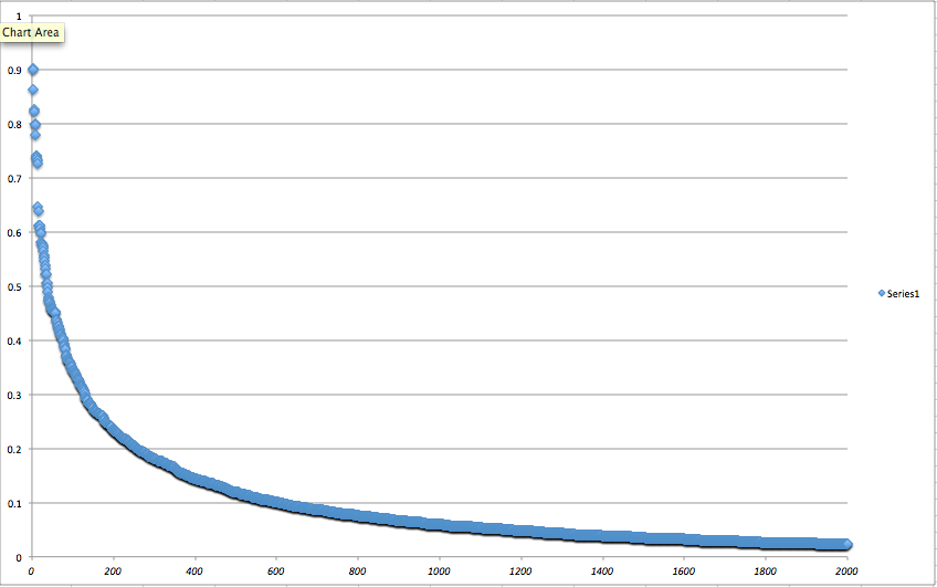
The Y-axis is the DF (document frequency), which varies from 0 to 1.0. The X-axis is just the term rank, from 1 (the term with the highest DF score, which is “the” in our example) down to 2000. This exhibits the happy power curve shape we’d expect. I typically pick a max DF score that’s right at the “elbow”, which is about 0.20 in the above graph. Interestingly enough, this 0.2 value is often the cut-off value for DF that I wind up using, regardless of the actual dataset being processed.

Now we can re-run the workflow, this time with the -maxdf 0.20 parameter and get a stop words list that we pass to the SolrAnalyzer constructor. We could automate the above process, by doing some curve fitting on the results and detecting the elbow, but for typical workflows the nature of the incoming data doesn’t change that much over time, so leaving it as a manual process is OK. I’ve added the list of stop words as src/main/resources/stopwords.txt. The last five terms in this file are:

fri
singl
those
expect
final

And those all seem reasonable to treat as stop words. Note that these are normalized (e.g. stemmed) terms, so you wouldn’t be able to directly use them as typical Solr/Lucene stop words. Instead the SolrAnalyzer code applies these against the analyzed results. In addition, this list wants to be language-specific. In fact much of the text processing (tokenizing, stemming, etc) should vary based on the language. Maybe that’s a topic for a future blog post series…

With our stop words list, we can regenerate results using the testStopwords() method in TextSimilarityWorkflowTest, which now look significantly better.

u_k	14.332966007716099
v_k	11.823697055234904
sgd	10.717215693020618
regress	10.58641818402347
categori	9.706156080342279
iri	9.675301677735192
u_k u_k	9.512846458340425
histori	8.913169188568189
dec	8.876447146205434
averag distanc	8.748071855787957

Filtering

At this point in the process we’re faced with a decision about second-stage filtering. Previously we’d filtered out noise (short words, numbers, stop words). Now we could do additional filtering to reduce the number of terms per document.

The first question is why might we want to do any filtering. The most common reason is one of performance – in general, fewer features mean better performance with machine learning algorithms, regardless of whether we’re doing k-means clustering or Solr-based real time similarity. Depending on what’s happening downstream, it might also make sense to reduce the amount of data we’re running through our workflow, which again is a performance win.

The second question is how to filter. There are lots of options, including:

• Picking a minimum LLR score (which might vary by the number of words in a term)
• Using a feature-reduction algorithm such as SVD (Singular Value Decomposition).
• Calculating a TF*IDF (Term frequency * inverse document frequency) score and taking only the top N.

It can also make sense to combine different types of filters – for example, to filter by a minimum LLR score initially to reduce the number of terms (workflow optimization), then calculate another score such as TF*IDF on the remaining terms.

In the next blog post, we’ll use TF*IDF to pick the best terms for each user, but we’ll do it in a way that is optimized for similarity. Stay tuned, I’ll try to get that written before I disappear for two weeks on the John Muir Trail.

Filed under:
Cascading, Machine Learning by kkrugler